Step 5: Analyze and Predict

Drivers: Step5_Analyze/Analyze.py, Step5_Analyze/Analyze_RRM.py Config: json_analyze.json

What this step does

Once Step 4 has identified a good (dataset, model) combination, Step 5 applies that trained model to prescribed data — a chosen time and region — to produce a fuel map.

Randomized versus prescribed data

This distinction runs through the whole pipeline:

	Randomized	Prescribed
Reference times	Many, sampled across 21 years	One — the time you want
Grid points	Randomly sampled	Every point in the chosen region
Purpose	Training and testing	Prediction

Prescribed data must be extracted and prepared exactly as the training data was — same max_history_to_consider, same history_interval, same quantities. A model trained on 41 features cannot be handed 61.

This is the lower path in the pipeline schematic on the home page.

Specifying what to predict

analysis_data_desired selects which raw data sources to run against, and each source gets a list of prediction requests:

"analysis_data_desired": ["SJSU", "HRRR", "RRM"],
"SJSU": [
    {
        "RefTime": "2018-11-08_22",
        "regions_x_indices": [[250, 390], [100, 250]],
        "regions_y_indices": [[100, 200], [300, 450]]
    },
    {
        "RefTime": "2020-09-04_00",
        "regions_x_indices": [[250, 390], [100, 250]],
        "regions_y_indices": [[100, 200], [300, 450]]
    }
]

RefTime is the prediction time in YYYY-MM-DD_HH format. The region lists give grid-index bounds, paired elementwise — the first x-range with the first y-range forms region 1, and so on. Regions may differ for each reference time.

Data sources

"raw_data": {
    "SJSU": "/p/vast1/climres/DFM_reanalysis",
    "HRRR": "/p/vast1/climres/hrrr_liner1/monthly",
    "RRM":  "/p/vast1/climres/E3SM/RRM"
}

Source	What it is
SJSU	The reanalysis dataset the models are trained on
HRRR	High-Resolution Rapid Refresh — operational weather, for near-term forecasts
RRM	E3SM regionally refined model — climate projections

Analyze_RRM.py is a separate driver for the RRM data, which has its own structure.

Predicting outside the training envelope

Trained models can be applied to times and places outside the training data, including future forecasts and climate scenarios. What makes this work is the variable mapping defined in Step 1 — as long as the new source has a counterpart for each quantity the model was trained on, it can be used.

Example output

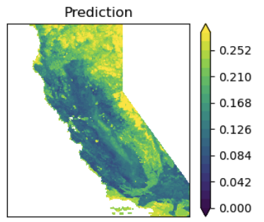
10-hour FM prediction for the entire state of California at 2018-11-08_22.

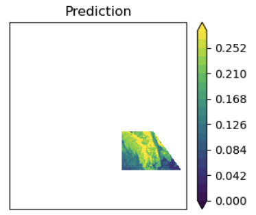
Sub-region 1

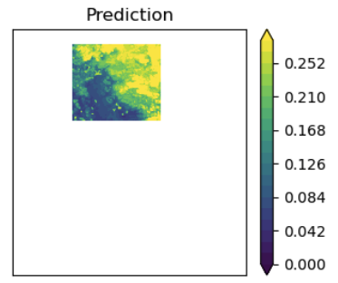
Sub-region 2

The date above is during the Woolsey Fire, one of the events named in the Step 1 fire_time_stamps block:

"fire_time_stamps": {
    "Woosley": {"Ref": "2018-11-08_22", "Start": "2018-11-01_00", "End": "2018-11-15_00"},
    "Creek":   {"Ref": "2020-09-04_00", "Start": "2020-08-28_00", "End": "2020-09-11_00"}
}

Output

Under analysis_data_base_loc, for each requested time and region:

• FM contour maps for the full domain and each sub-region
• Scatter plots of prediction against ground truth, where ground truth exists

Ground-truth comparison is only possible for sources that carry FM values — reanalysis data does, forecasts and projections do not. For those, the fuel map is the product.