Step 4: Evaluate Models

Driver: Step4_EvalModels/EvaluateTrainedModels.py Config: json_eval_sample.json

What this step does

Step 3 evaluates one (dataset, label, model) combination. Step 4 collects many of them into a collection matrix and produces comparative heatmaps and bar plots, so you can see which combinations perform best.

This is where a parametric study becomes interpretable.

The collection matrix

The matrix has two axes.

Axis 1 — datasets. json_extract_counts lists the Step 1 dataset identifiers to include:

"json_extract_counts": [39, 40, 41, 42, 43, 44, 45, 46, 47, 48, 49,
                        51, 52, 53, 55, 56, 59, 60, 61, 62, 63, 64, 65, 66]

Axis 2 — (label, model) pairs. json_prep_train_maps gives groups of label and model identifiers, with human-readable descriptions used as plot legends:

"json_prep_train_maps": [
    {
        "json_label": [6],
        "json_train": [3, 6, 7, 8],
        "set_info": ["UMag10, T2, RH"],
        "subset_info": ["PREC, SW", "PREC", "SW", ""]
    },
    {
        "json_label": [6],
        "json_train": [9, 10, 11, 12],
        "set_info": ["HGT, UMag10, T2, RH"],
        "subset_info": ["PREC, SW", "PREC", "SW", ""]
    }
]

Read the first group as: label configuration 6, trained four ways (3, 6, 7, 8), all using the base feature set UMag10, T2, RH, with the four variants adding PREC, SW, then PREC only, then SW only, then neither.

set_info and subset_info are purely descriptive — they label the plots. They must correspond to what the referenced training configurations actually do; nothing verifies this for you.

Metrics and sets

"metric_names": ["r2_score", "ev_score", "mse", "rmse", "max_err", "mae", "medae"],
"metric_on_sets": ["train", "test", "test_p90", "test_p95"]

Seven metrics across four datasets produces 28 combinations, and each yields both a heatmap and a bar plot — 56 plots per collection.

For classification problems, accuracy is the only metric; everything else is identical.

Locating the input files

Step 4 does not take the earlier JSON files as arguments. It reconstructs their paths from a base directory plus the identifier lists:

"paths": {
    "eval_model_base_loc": ".../04_Eval_Models",
    "sim_dir": ".../Wildfire_LDRD_SI",
    "json_extract_base": "InputJson/Extract/json_extract_data",
    "json_prep_base": "InputJson/Prep/json_prep_data_label",
    "json_train_base": "InputJson/Train/json_train_model"
}

Identifier 39 under json_extract_base resolves to <sim_dir>/InputJson/Extract/json_extract_data_039.json. Identifiers are zero-padded to three digits.

This means your JSON files must be organized in that directory layout for Step 4 to find them. See Running on HPC.

Naming the collection

"evaluation": {
    "count": 1,
    "identifier_text": "many_cases"
}

These combine into the output directory name — eval_001_many_cases. Choosing a descriptive identifier_text is what makes a large study navigable months later; the published studies use names like temporal_data_effect and RF_estimator_effect.

Example outputs

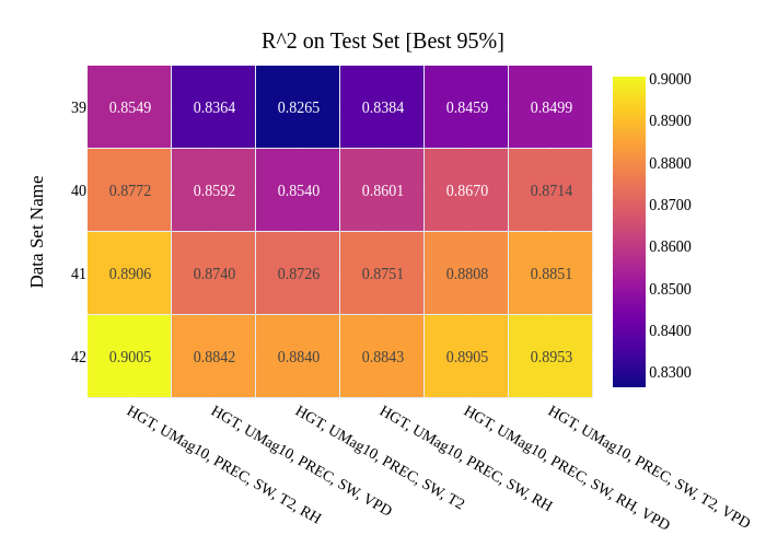
R² on test data (best 95%) for several datasets and models.

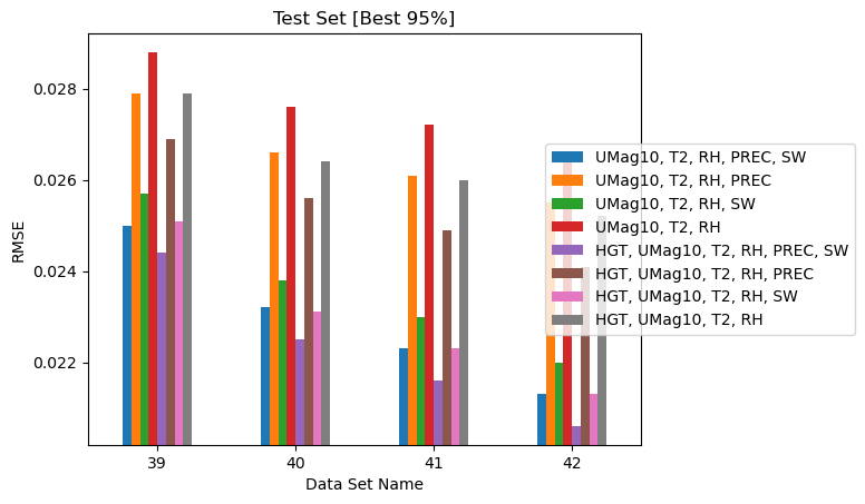
Root mean squared error on test data (best 95%) for a collection of datasets and models.

Output

Per collection, under eval_model_base_loc:

• 56 plots — a heatmap and bar plot for each metric/dataset pair
• Matching CSV files with the underlying numbers
• <collection>_data_defn.csv recording the parameters defining each dataset in the collection

The CSVs are the authoritative record; every result in the Science with MLAP section is drawn from them.