Step 3: Train Models
Driver: Step3_TrainModel/TrainModel.py
Config: json_train_model_<MODEL>.json
What this step does
Step 3 scales the prepared data, splits it into train and test sets, fits a model, and computes evaluation metrics and plots for that single (dataset, label, model) combination.
Comparing many such combinations is Step 4.
Training options
| Parameter | Effect |
|---|---|
train_from_scratch |
true fits a new model; false loads an already-trained model matching the nomenclature and evaluates it |
save_train_data |
Retain the training split for later examination |
save_test_data |
Retain the test split for later examination |
Setting train_from_scratch to false is how you re-evaluate or re-plot without
paying to retrain.
Scaling
Features arrive on wildly different scales — wind speed sits around \([0, 15]\) m/s while temperature (WRF outputs Kelvin − 300) runs \([-50, 20]\). Without scaling, distance-based and gradient-based models are dominated by whichever feature happens to have the largest numeric range.
scaler_type selects the scikit-learn scaler:
| Value | Scaler |
|---|---|
"Standard" |
StandardScaler — zero mean, unit variance |
"MinMax" |
MinMaxScaler — rescale to a fixed range |
"MaxAbs" |
MaxAbsScaler — scale by maximum absolute value |
"Robust" |
RobustScaler — uses median and IQR, resistant to outliers |
An unrecognized value raises a ValueError rather than silently defaulting.
Which scaler to pick is examined in ML Parameters.
Train/test split
test_data_frac sets the fraction held out for testing. 0.2 means 20% test,
80% train.
Available models
model_name selects the algorithm. The regression or classification variant is
chosen automatically from the label_type set in
Step 2.
model_name |
Regression | Classification |
|---|---|---|
"Linear" |
LinearRegression |
— |
"SVM" |
SVR |
SVC |
"RF" |
RandomForestRegressor |
RandomForestClassifier |
"MLP" |
MLPRegressor |
MLPClassifier |
"GB" |
GradientBoostingRegressor |
GradientBoostingClassifier |
"Linear" has no classification counterpart. The framework is straightforward to
extend with additional models.
Model hyperparameters
By default models use scikit-learn defaults. params overrides them, passed
through directly to the model constructor:
"models": {
    "model_name": "MLP",
    "params": {
        "hidden_layer_sizes": [15, 15],
        "activation": "relu",
        "solver": "adam",
        "alpha": 0.0001,
        "learning_rate": "constant",
        "learning_rate_init": 0.001,
        "max_iter": 500,
        "shuffle": true,
        "tol": 1e-3
    }
}
An empty "params": {} means "use scikit-learn defaults" — that is what the
Random Forest configuration in the repository does.
The effect of these choices is documented in ML Parameters.
Choosing features for training
The prepared data may carry a wide master list of features, but training can use
any subset via qois_for_training:
"features_labels": {
    "qois_for_training": ["UMag10", "T2", "RH", "PREC", "SW"],
    "label_log": false
}
Given prepared data containing
["HGT", "UMag10", "T2", "RH", "VPD", "PREC", "SW"], you might train on:
["HGT", "UMag10", "T2", "RH"]["HGT", "UMag10", "T2", "VPD", "PREC", "SW"]["HGT", "UMag10", "T2", "VPD", "PREC"]
This is the mechanism behind the feature-importance studies in Physical Quantities — you prepare the data once and vary only this list.
Evaluation datasets
Metrics are computed on four sets:
| Dataset | Definition |
|---|---|
train |
Training data, e.g. 80% of prepared data after scaling |
test |
Test data, e.g. 20% of prepared data after scaling |
test_p95 |
Best 95% of test data, ranked by prediction error |
test_p90 |
Best 90% of test data, ranked by prediction error |
Comparing train against test exposes overfitting. The p95 and p90 sets
exist because a small number of outliers can dominate an aggregate metric and
obscure how the model performs on the bulk of the data.
Note
These are computed on predictions, and are distinct from
prune_data, which removes rows before
training.
Regression metrics
All seven are computed on all four datasets, giving 28 numbers per (dataset, label, model) combination:
| Metric | Definition |
|---|---|
r2_score |
R-squared |
ev_score |
Explained variance score |
mse |
Mean squared error |
rmse |
Root mean squared error |
max_err |
Maximum error |
mae |
Mean absolute error |
medae |
Median absolute error |
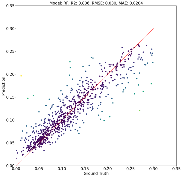
Entire test dataset
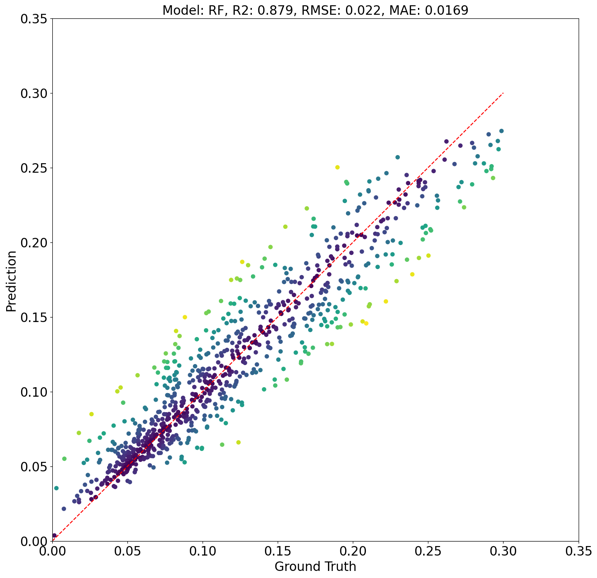
Best 95% of test data
Ground truth against prediction for a regression problem using Random Forest. Darker colors are smaller errors; selected metrics appear in the title.
Classification metrics
Classification problems use accuracy as the primary metric, visualized with a confusion matrix. Everything else about the step is unchanged.
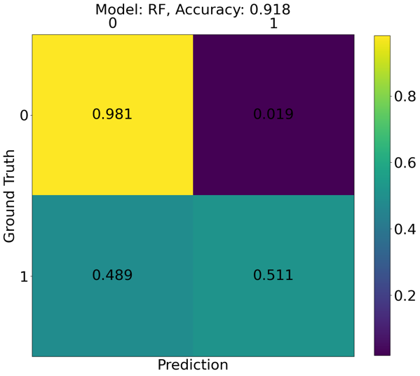
Binary, FM_binary_threshold = 0.05
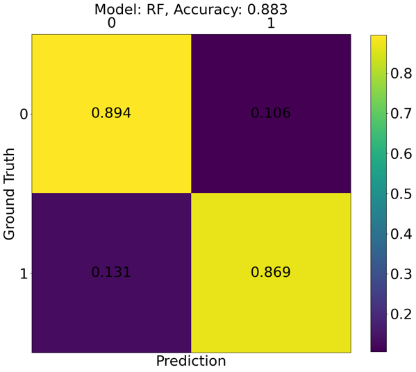
Binary, FM_binary_threshold = 0.10
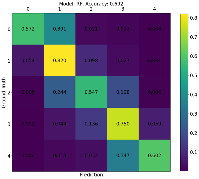
Multi-class confusion matrix for FM_MC_levels =
[0.0, 0.05, 0.10, 0.15, 0.25, 1.0], 10-hour fuel moisture.
Plot appearance
The evaluation block controls figure rendering:
"evaluation": {
    "max_data_size_scatter": 800,
    "fig_size_x": 15,
    "fig_size_y": 15,
    "font_size": 20,
    "x_lim": [0, 0.35],
    "normalize_cm": true
}
max_data_size_scatter caps how many points are drawn in scatter plots — it
affects the figure only, not the metrics. normalize_cm normalizes the confusion
matrix.
Output
A trained model, its metrics as CSV, and scatter or confusion-matrix plots,
written under trained_model_base_loc and named by the
(dataset, label, model) nomenclature.